Mapping GPS data from our USA/ Canada Roadtrip
This September we went on a roadtrip to the US and Canada. Of course, we had our trusty GPS to guide us along the way - the data from which I downloaded and used to play around with.
(If you want to see a few photos from the trip and don’t care about the rest, skip to the bottom…)
Loading the data
I used the XML package to load the gpx files following this blog post.
library(XML)

myfiles <- list.files(path = "../gpx/gpx_files", full.names = TRUE)

for (i in 1:length(myfiles)){

  # One of the files seems to be broken, but since the file is one with earlier data
  # not from the trip, I will simply skip it
  tryCatch({
    pfile <- htmlTreeParse(myfiles[i], useInternalNodes = T)

  }, error=function(e){cat("ERROR\n")})

  if (exists("pfile")){
    # Get all elevations, times and coordinates via the respective xpath
    elevations <- as.numeric(as.character(xpathSApply(pfile, path = "//trkpt/ele", xmlValue)))
    times <- xpathSApply(pfile, path = "//trkpt/time", xmlValue)
    coords <- xpathSApply(pfile, path = "//trkpt", xmlAttrs)
    # Extract latitude and longitude from the coordinates
    lats <- as.numeric(as.character(coords["lat",]))
    lons <- as.numeric(as.character(coords["lon",]))
    # Put everything in a dataframe and get rid of old variables
    geodf <- data.frame(lat = lats, lon = lons, ele = elevations, time = times)

    if (i == 1){
      geodata <- geodf
      } else {
      geodata <- rbind(geodata, geodf)
    }
  }
  rm(pfile)
}
geodata_all <- geodata
I then did some cleaning of the date and time column and removed all the old track that were not part of our trip.
# Transforming the time column
geodata_all$time <- strptime(geodata_all$time, format = "%Y-%m-%dT%H:%M:%SZ")

# ordering by date
library(plyr)
geodata_all <- arrange(geodata_all, time)

# removing all tracks from Germany
geodata <- geodata_all[which(as.numeric(as.character(geodata_all$lon)) < 0),]

# adding a column with day for separating the plotting by day lateron
geodata$day <- as.factor(format(as.Date(geodata$time,format="%Y-%m-%d"), "%d"))
We have 119225 data points with a range from 2016-09-09 19:23:53 to 2016-09-23 21:36:06.
summary(geodata)
##       lat             lon              ele
##  Min.   :36.99   Min.   :-88.68   Min.   :-26.78
##  1st Qu.:40.09   1st Qu.:-84.86   1st Qu.:181.83
##  Median :41.90   Median :-82.99   Median :198.65
##  Mean   :41.27   Mean   :-82.76   Mean   :216.58
##  3rd Qu.:42.33   3rd Qu.:-80.44   3rd Qu.:255.85
##  Max.   :43.65   Max.   :-78.85   Max.   :438.02
##
##       time                          day
##  Min.   :2016-09-09 19:23:53   19     :17203
##  1st Qu.:2016-09-12 12:14:47   12     :14455
##  Median :2016-09-15 21:52:37   11     :14020
##  Mean   :2016-09-15 22:35:18   10     :12061
##  3rd Qu.:2016-09-19 15:59:09   16     :10856
##  Max.   :2016-09-23 21:36:06   13     :10787
##                                (Other):39843
str(geodata)
## 'data.frame':    119225 obs. of  5 variables:
##  $ lat : num  42 42 42 42 42 ...
##  $ lon : num  -87.9 -87.9 -87.9 -87.9 -87.9 ...
##  $ ele : num  122 122 122 122 122 ...
##  $ time: POSIXlt, format: "2016-09-09 19:23:53" "2016-09-09 19:23:53" ...
##  $ day : Factor w/ 15 levels "09","10","11",..: 1 1 1 1 1 1 1 1 1 1 ...
Getting additional data from Google Maps
Somehow the GPS didn’t record the last two days of our trip back to Chicago, so I added a few way points with the Google Maps Geocoding and Directions APIs (accessed via the googleway package).
library(googleway)

# on th 26th we had lunch at cracker barrel
cracker_barrel <- google_geocode(address = "2101 N Kenyon Rd, Urbana, IL 61802, USA",
                                 key = "your_key",
                                 language = "en",
                                 simplify = TRUE)

cracker_barrel_data <- data.frame(lat = cracker_barrel$results$geometry$location$lat,
                                  lon = cracker_barrel$results$geometry$location$lng,
                                  ele = "NA", time = as.POSIXlt("2016-09-26 19:00:00"))

# then we stayed the night in Aurora/ Naperville
super8 <- google_geocode(address = "4228 Longmeadow Dr, Aurora, IL 60504, USA",
                         key = "your_key",
                         language = "en",
                         simplify = TRUE)

super8_data <- data.frame(lat = super8$results$geometry$location$lat,
                          lon = super8$results$geometry$location$lng,
                          ele = "NA", time = as.POSIXlt("2016-09-26 23:30:00"))

# on the 27th we went back to the airport to fly home
ohare <- google_geocode(address = "10000 W O'Hare Ave, Chicago, IL 60666, USA",
                        key = "your_key",
                        language = "en",
                        simplify = TRUE)

ohare_data <- data.frame(lat = ohare$results$geometry$location$lat,
                         lon = ohare$results$geometry$location$lng,
                         ele = "NA", time = as.POSIXlt("2016-09-27 18:00:00"))
Using only these three waypoints won’t plot nicely on a map because it will draw straight lines between the points. So, I also want to get travel information from Google Maps between these points to get a few more waypoints along the actual route we drove.
## Route from Paducah to Cracker Barrel

route_pad_cracker <- google_directions(origin = c(geodata$lat[nrow(geodata)], geodata$lon[nrow(geodata)]),
                  destination = c(cracker_barrel_data$lat, cracker_barrel_data$lon),
                  mode = "driving",
                  key = "your_key",
                  language = "en",
                  simplify = TRUE)

route_pad_cracker_legs <- as.data.frame(route_pad_cracker$routes$legs)
route_pad_cracker_legs_steps <- as.data.frame(route_pad_cracker_legs$steps)

## Route from Cracker Barrel to Aurora

route_cracker_aurora <- google_directions(origin = c(cracker_barrel_data$lat, cracker_barrel_data$lon),
                                          destination = c(super8_data$lat, super8_data$lon),
                                          mode = "driving",
                                          key = "your_key",
                                          language = "en",
                                          simplify = TRUE)

route_cracker_aurora_legs <- as.data.frame(route_cracker_aurora$routes$legs)
route_cracker_aurora_legs_steps <- as.data.frame(route_cracker_aurora_legs$steps)

## Route from Cracker Aurora to O'Hare

route_aurora_ohare <- google_directions(origin = c(super8_data$lat, super8_data$lon),
                                        destination = c(ohare_data$lat, ohare_data$lon),
                                        mode = "driving",
                                        key = "your_key",
                                        language = "en",
                                        simplify = TRUE)

route_aurora_ohare_legs <- as.data.frame(route_aurora_ohare$routes$legs)
route_aurora_ohare_legs_steps <- as.data.frame(route_aurora_ohare_legs$steps)

# Combining the data sets
geodata_2 <- data.frame(lat = c(geodata$lat,
                                route_pad_cracker_legs$start_location$lat, route_pad_cracker_legs_steps$start_location$lat,
                                route_pad_cracker_legs$end_location$lat, cracker_barrel_data$lat,
                                route_cracker_aurora_legs$start_location$lat, route_cracker_aurora_legs_steps$start_location$lat,
                                route_cracker_aurora_legs$end_location$lat, super8_data$lat,
                                route_aurora_ohare_legs$start_location$lat, route_aurora_ohare_legs_steps$start_location$lat,
                                route_aurora_ohare_legs$end_location$lat, ohare_data$lat),
                      lon = c(geodata$lon, route_pad_cracker_legs$start_location$lng, route_pad_cracker_legs_steps$start_location$lng,
                              route_pad_cracker_legs$end_location$lng, cracker_barrel_data$lon,
                              route_cracker_aurora_legs$start_location$lng, route_cracker_aurora_legs_steps$start_location$lng,
                              route_cracker_aurora_legs$end_location$lng, super8_data$lon,
                              route_aurora_ohare_legs$start_location$lng, route_aurora_ohare_legs_steps$start_location$lng,
                              route_aurora_ohare_legs$end_location$lng, ohare_data$lon),
                      day = c(as.character(geodata$day), rep("26",
                                               length(c(route_pad_cracker_legs$start_location$lat,
                                                        route_pad_cracker_legs_steps$start_location$lat,
                                                        route_pad_cracker_legs$end_location$lat, cracker_barrel_data$lat,
                                                        route_cracker_aurora_legs$start_location$lat,
                                                        route_cracker_aurora_legs_steps$start_location$lat,
                                                        route_cracker_aurora_legs$end_location$lat, super8_data$lat))),
                              rep("27",
                                  length(c(route_aurora_ohare_legs$start_location$lat, route_aurora_ohare_legs_steps$start_location$lat,
                                           route_aurora_ohare_legs$end_location$lat, ohare_data$lat)))))
Plotting
I tried several packages for plotting but ended up with ggmap as the nicest looking solution.
Overview of the trip
We flew to Chicago, went west across Michigan to Ann Arbor, Detroit, Toronto, then south again to Pittsburgh, from where we followed the Ohio river and headed to Louisville. From there, we went to Paducah, KY and back north again to Chicago. Each color shows a different day.
library(ggmap)

bc_bbox <- make_bbox(lat = lat, lon = lon, data = geodata_2, f = .10)
map <- get_map(location = bc_bbox, maptype = "roadmap")

ggmap(map, darken = c(0.3, "white")) + geom_point(aes(x = lon, y = lat, col = factor(day), group = factor(day)), data = geodata_2) +
  geom_path(aes(x = lon, y = lat, col = factor(day)), data = geodata_2[which(geodata_2$day %in% c("26", "27")), ]) +
  theme(legend.position="none") + labs(x="Longitude", y="Latitude", title="Roadtrip 2016")
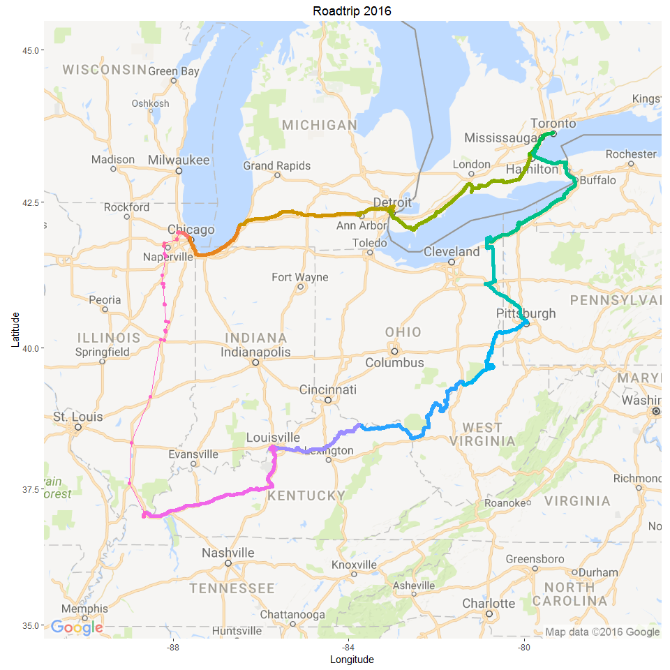
Road trip with stops
First, I need to obtain the geocodes from the stops (again via Google Maps API).
chicago <- google_geocode(address = "Chicago",
                          key = "your_key",
                          language = "en",
                          simplify = TRUE)

stjospeh <- google_geocode(address = "St. Joseph, MI",
                          key = "your_key",
                          language = "en",
                          simplify = TRUE)

annarbor <- google_geocode(address = "Ann Arbor, MI",
                           key = "your_key",
                           language = "en",
                           simplify = TRUE)

detroit <- google_geocode(address = "Detroit, MI",
                           key = "your_key",
                           language = "en",
                           simplify = TRUE)

burlington <- google_geocode(address = "Burlington, ON",
                          key = "your_key",
                          language = "en",
                          simplify = TRUE)

ashtabula <- google_geocode(address = "Ashtabula",
                             key = "your_key",
                             language = "en",
                             simplify = TRUE)

pittsburgh <- google_geocode(address = "Pittsburgh",
                            key = "your_key",
                            language = "en",
                            simplify = TRUE)

marietta <- google_geocode(address = "Marietta, OH",
                             key = "your_key",
                             language = "en",
                             simplify = TRUE)

maysville <- google_geocode(address = "Maysville, KY",
                             key = "your_key",
                             language = "en",
                             simplify = TRUE)

louisville <- google_geocode(address = "Louisville, KY",
                             key = "your_key",
                             language = "en",
                             simplify = TRUE)

paducah <- google_geocode(address = "Paducah, KY",
                             key = "your_key",
                             language = "en",
                             simplify = TRUE)

ann_text <- data.frame(x = c(chicago$results$geometry$location$lng,
                             stjospeh$results$geometry$location$lng,
                             annarbor$results$geometry$location$lng,
                             detroit$results$geometry$location$lng,
                             burlington$results$geometry$location$lng,
                             ashtabula$results$geometry$location$lng,
                             pittsburgh$results$geometry$location$lng,
                             marietta$results$geometry$location$lng,
                             maysville$results$geometry$location$lng,
                             louisville$results$geometry$location$lng[1], #Maps found a second entry for the location
                             paducah$results$geometry$location$lng),
                       y = c(chicago$results$geometry$location$lat,
                             stjospeh$results$geometry$location$lat,
                             annarbor$results$geometry$location$lat,
                             detroit$results$geometry$location$lat+0.1, #adjusting Detroit label to avoid overlapping with Ann Arbor
                             burlington$results$geometry$location$lat,
                             ashtabula$results$geometry$location$lat,
                             pittsburgh$results$geometry$location$lat,
                             marietta$results$geometry$location$lat,
                             maysville$results$geometry$location$lat,
                             louisville$results$geometry$location$lat[1],
                             paducah$results$geometry$location$lat),
                       labs = c(paste0(chicago$results$formatted_address),
                                paste0(stjospeh$results$formatted_address),
                                paste0(annarbor$results$formatted_address),
                                paste0(detroit$results$formatted_address),
                                paste0(burlington$results$formatted_address),
                                paste0(ashtabula$results$formatted_address),
                                paste0(pittsburgh$results$formatted_address),
                                paste0(marietta$results$formatted_address),
                                paste0(maysville$results$formatted_address),
                                paste0(louisville$results$formatted_address[1]),
                                paste0(paducah$results$formatted_address)
                                ))
map <- get_map(location = bc_bbox, maptype = "watercolor")

roadtrip_map <- ggmap(map, darken = c(0.3, "white")) + geom_point(aes(x = lon, y = lat, col = factor(day), group = factor(day)), data = geodata_2, alpha = 0.3) +
  geom_path(aes(x = lon, y = lat, col = factor(day)), data = geodata_2[which(geodata_2$day %in% c("26", "27")), ], alpha = 0.5) +
  theme(legend.position="none") + labs(x="Longitude", y="Latitude", title="Roadtrip 2016")
roadtrip_map + geom_text(data = ann_text, aes(x, y, label = labs), size = 4)
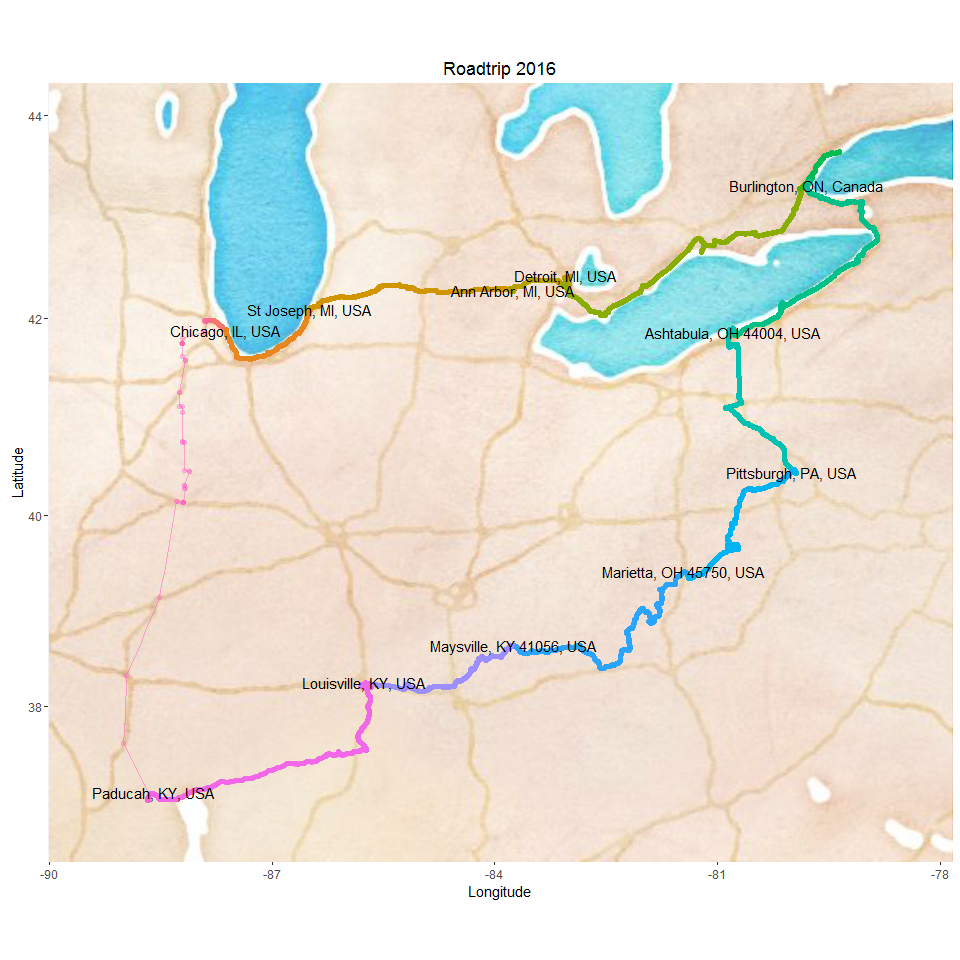
Road trip statistics
How many kilometers did we drive?
# removing duplicate entries
geodata_2 <- geodata_2[!duplicated(geodata_2), ]

# Shifting vectors for latitude and longitude to include end position
shift.vec <- function (vec, shift){
  if(length(vec) <= abs(shift)){
    rep(NA ,length(vec))
  } else {
    if (shift >= 0) {
      c(rep(NA, shift), vec[1:(length(vec)-shift)]) }
    else {
      c(vec[(abs(shift)+1):length(vec)], rep(NA, abs(shift)))
    }
  }
}

geodata_2$lat.p1 <- shift.vec(geodata_2$lat, -1)
geodata_2$lon.p1 <- shift.vec(geodata_2$lon, -1)

# Calculating distances between points (in metres) with the function pointDistance from the 'raster' package.

library(raster)
geodata_2$dist.to.prev <- apply(geodata_2, 1, FUN = function (row) {
  pointDistance(c(as.numeric(as.character(row["lat.p1"])),
                  as.numeric(as.character(row["lon.p1"]))),
                c(as.numeric(as.character(row["lat"])), as.numeric(as.character(row["lon"]))),
                lonlat = T) # Parameter 'lonlat' has to be TRUE!
})
We drove approximately 3236.95 km in 18 days. Not counting the ~6 days where we stayed in one place and didn’t drive much, that’s around 269.75 km/ day.
Identifying local time
The time stamps are in CEST - Central European Summer Time. We arrived in the Central Time Zone (CDT) but spent the majority of our trip in Estern Time Zone (EDT).
Converting to CDT and EDT
library(lubridate)

geodata$time_CDT <- with_tz(geodata$time, tz="America/Chicago")
geodata$time_EDT <- with_tz(geodata$time, tz="America/New_York")

# extracting day for EDT
geodata$day_EDT <- as.factor(format(as.Date(geodata$time_EDT,format="%Y-%m-%d"), "%d"))
Identifying the local time based on geocode
# the days where we crossed time zones were the 10th and 23rd

library(googleway)

geodata_timezone <- geodata
geodata_timezone$local_time <- "NA"

for (i in 1:nrow(geodata)){
  if (is.na(nchar(strsplit(as.character(i/100), "\\.")[[1]][2]))){
    print(i)
  }

  if (geodata[i, "day_EDT"] == "10"){
    data_row <- geodata[i, ]
    google_timezone_api <- google_timezone(location = c(data_row$lat, data_row$lon),
                                           timestamp = as.POSIXct(data_row$time_EDT), # because the majority of our trip was in EDT
                                           key = "AIzaSyBkqrk8mBqqvao-W-jKkL2VhHCGLWqZVCY",
                                           simplify = TRUE,
                                           language = "en")

    time_zone <- google_timezone_api$timeZoneId

    local_time <- as.POSIXlt(with_tz(data_row$time, tz=paste(time_zone)))

    geodata_timezone$local_time[i] <- as.character(local_time)

    rm(data_row, google_timezone_api, time_zone)

  } else {

    if (geodata[i, "day_EDT"] == "09"){
      geodata_timezone$local_time[i] <- as.character(geodata_timezone$time_CDT[i])
    } else {
      geodata_timezone$local_time[i] <- as.character(geodata_timezone$time_EDT[i])
    }
  }
}
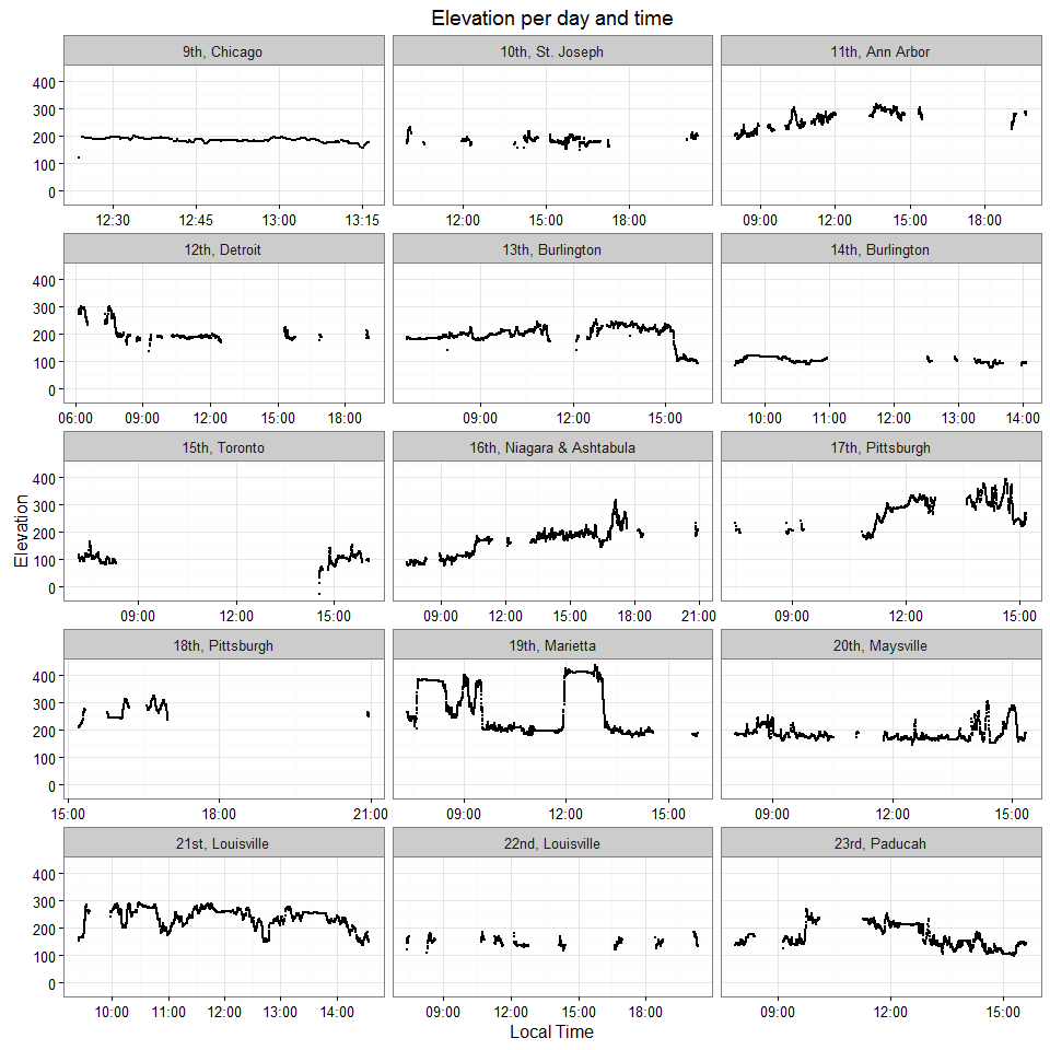
Plotting elevation
theme_set(theme_bw()) # Change the theme to my preference

labels <- c("9" = "9th, Chicago", "10" = "10th, St. Joseph", "11" = "11th, Ann Arbor", "12" = "12th, Detroit", "13" = "13th, Burlington",
            "14" = "14th, Burlington", "15" = "15th, Toronto", "16" = "16th, Niagara & Ashtabula", "17" = "17th, Pittsburgh",
            "18" = "18th, Pittsburgh", "19" = "19th, Marietta", "20" = "20th, Maysville", "21" = "21st, Louisville",
            "22" = "22nd, Louisville", "23" = "23rd, Paducah")

ggplot(aes(x = as.POSIXlt(local_time), y = ele), data = geodata_timezone) +
  geom_point(size = 0.5) + facet_wrap( ~ day_EDT, ncol=3, scales = "free_x", labeller=labeller(day_EDT = labels)) +
  labs(x="Local Time", y="Elevation", title="Elevation per day and time")
day_df <- data.frame(row.names = unique(geodata_timezone$day_EDT),
                     group = unique(geodata_timezone$day_EDT),
                     xmin = rep(NA, length(unique(geodata_timezone$day_EDT))),
                     xmax = rep(NA, length(unique(geodata_timezone$day_EDT))),
                     ymin = rep(-Inf, length(unique(geodata_timezone$day_EDT))),
                     ymax = rep(Inf, length(unique(geodata_timezone$day_EDT))))

for (day in unique(geodata_timezone$day_EDT)){
  if (!day == "23"){
    day_df[paste(day), 2] <- which(geodata_timezone$day_EDT == day)[1]
    day_df[paste(day), 3] <- which(geodata_timezone$day_EDT == as.numeric(as.character(day))+1)[1]-1
  } else {
    day_df[paste(day), 2] <- which(geodata_timezone$day_EDT == day)[1]
    day_df[paste(day), 3] <- nrow(geodata_timezone)
  }
}

ggplot(aes(x = seq_along(ele), y = ele), data = geodata_timezone) +
  geom_rect(data=day_df, inherit.aes=FALSE,
           aes(xmin=xmin, xmax=xmax, ymin=ymin, ymax=ymax, fill = factor(group)), col = "grey", alpha=0.5) +
  #annotate("rect", xmin=0, xmax=0, ymin=-Inf, ymax=0, fill="red", alpha=0.5) +
  geom_path() +
  labs(x="Index", y="Elevation (line) and day (rectangles)", title="Elevation per day") +
  scale_y_continuous(limits = c(min(c(geodata_timezone$ele, as.numeric(as.character(geodata_timezone$day_EDT)))),
                                max(c(geodata_timezone$ele, as.numeric(as.character(geodata_timezone$day_EDT)))))) +
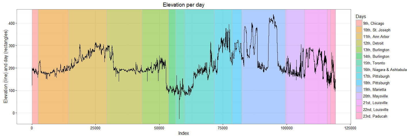
  scale_fill_discrete(name="Days", labels = labels)
Extracting speed data from the gpx files
Looking at the gpx file, there is also speed and course data. It is saved into the extensions tag. However, not all data points seem to have a speed tag.
for (i in 1:length(myfiles)){

  tryCatch({
    singleString <- paste(readLines(myfiles[i]), collapse=" ")
    pfile2 <- gsub("</time><extensions><gpxtpx:TrackPointExtension><gpxtpx:course>",
                   "</time><extensions><gpxtpx:TrackPointExtension><gpxtpx:speed>0.00</gpxtpx:speed><gpxtpx:course>", singleString)

    pfile <- htmlTreeParse(pfile2, useInternalNodes = T)

    # Get all elevations, times and coordinates via the respective xpath
    times <- xpathSApply(pfile, path = "//trkpt/time", xmlValue)
    coords <- xpathSApply(pfile, path = "//trkpt", xmlAttrs)
    # Extract latitude and longitude from the coordinates
    lats <- as.numeric(as.character(coords["lat",]))
    lons <- as.numeric(as.character(coords["lon",]))

    speed <- xpathSApply(pfile, path = "//trkpt/extensions/*/speed", xmlValue)# in m/s

    # course gives the degrees where the car was headed at that point
    course <- xpathSApply(pfile, path = "//trkpt/extensions/*/course", xmlValue)
    # Put everything in a dataframe and get rid of old variables
    geodf <- data.frame(lat = lats, lon = lons, time = times, speed = speed, course = course)

    if (i == 1){
      geodata_new <- geodf
    } else {
      geodata_new <- rbind(geodata_new, geodf)
    }

    rm(pfile, pfile2, singleString)
  }, error=function(e){cat("ERROR\n")})

}
# Transforming the time column
geodata_new$time <- strptime(geodata_new$time, format = "%Y-%m-%dT%H:%M:%SZ")

# ordering by date
geodata_new <- arrange(geodata_new, time)

# removing all tracks from Germany
geodata_new_trip <- geodata_new[which(as.numeric(as.character(geodata_new$lon)) < 0),]

# adding a column with day for separating the plotting by day lateron
geodata_new_trip$day <- as.factor(format(as.Date(geodata_new_trip$time,format="%Y-%m-%d"), "%d"))

head(geodata_new_trip)
##            lat      lon                time speed course day
## 35664 41.98135 -87.8818 2016-09-09 19:23:53  0.00   0.00  09
## 35665 41.98135 -87.8818 2016-09-09 19:23:53  0.00   0.00  09
## 35666 41.98135 -87.8818 2016-09-09 19:23:53  0.00   0.00  09
## 35667 41.98135 -87.8818 2016-09-09 19:23:53  0.00   0.00  09
## 35668 41.98135 -87.8818 2016-09-09 19:23:53  0.00   0.00  09
## 35669 41.98135 -87.8818 2016-09-09 19:23:53  0.00   0.00  09
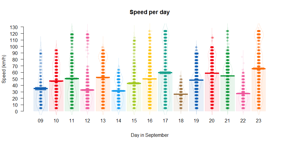
Garmin shows speed as m/s, so I am converting it to km/h.
library(yarrr)

geodata_new_trip$speed_kmh <- as.numeric(as.character(geodata_new_trip$speed)) *3.6

speed_data <- geodata_new_trip[which(as.numeric(as.character(geodata_new_trip$speed_kmh)) > 0),]
speed_data <- speed_data[!duplicated(speed_data), ]

summary(as.numeric(as.character(speed_data$speed_kmh)))
##    Min. 1st Qu.  Median    Mean 3rd Qu.    Max.
##   4.932  24.700  44.460  49.210  69.190 128.500
pirateplot(formula = as.numeric(as.character(speed_kmh)) ~ as.factor(day),
           point.o = .1,
           data = speed_data,
           ylab = "Speed (km/h)",
           xlab = "Day in September",
           main = "Speed per day")
Photos
And finally some photos from our trip. Their locations are marked on the map below:
myphotos <- list.files(path = ".", full.names = TRUE)
myphotos <- myphotos[grep("jpg", myphotos)]

library(exif)

photo_geotags <- data.frame(row.names = gsub("./", "", myphotos), lat = rep(NA, length(myphotos)), lon = NA)

for (file in gsub("./", "", myphotos)){
  photodata <- read_exif(file)
  lat <- photodata$latitude
  lon <- photodata$longitude
  photo_geotags[file, ]$lat <- lat
  photo_geotags[file, ]$lon <- lon
}

photo_geotags$text <- seq(1:nrow(photo_geotags))

library(ggmap)
library(ggrepel)

bc_bbox <- make_bbox(lat = lat, lon = lon, data = photo_geotags, f = .10)
map <- get_map(location = bc_bbox, maptype = "roadmap")

ggmap(map, darken = c(0.3, "white")) +
  geom_point(aes(x = lon, y = lat), data = photo_geotags) +
  theme(legend.position="none") + labs(x="Longitude", y="Latitude", title="Roadtrip 2016") +
  geom_text_repel(aes(label = text), data = photo_geotags)
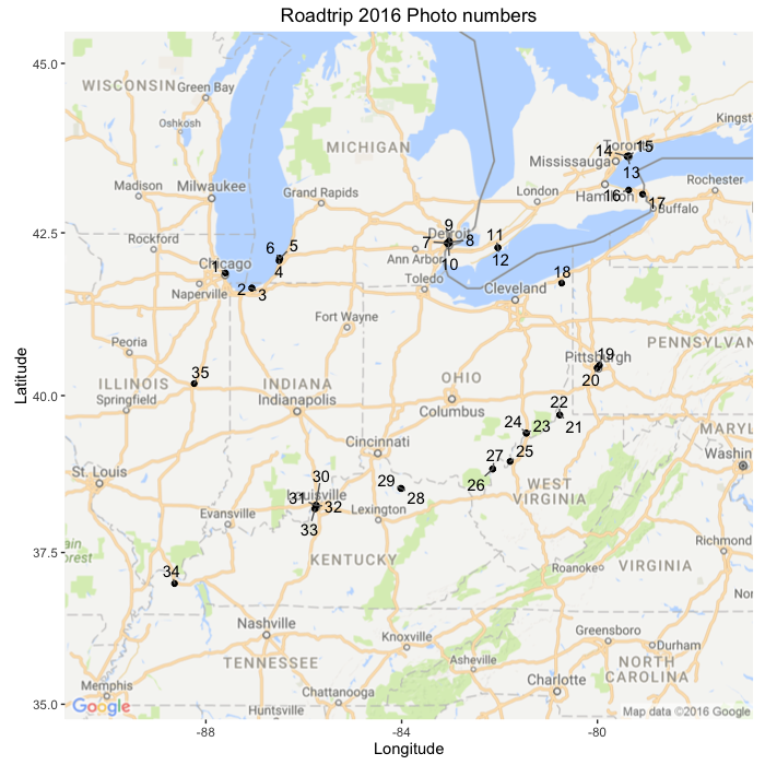
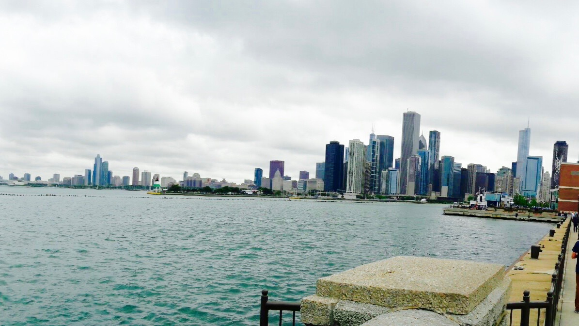 Photo number 1
 Photo number 2
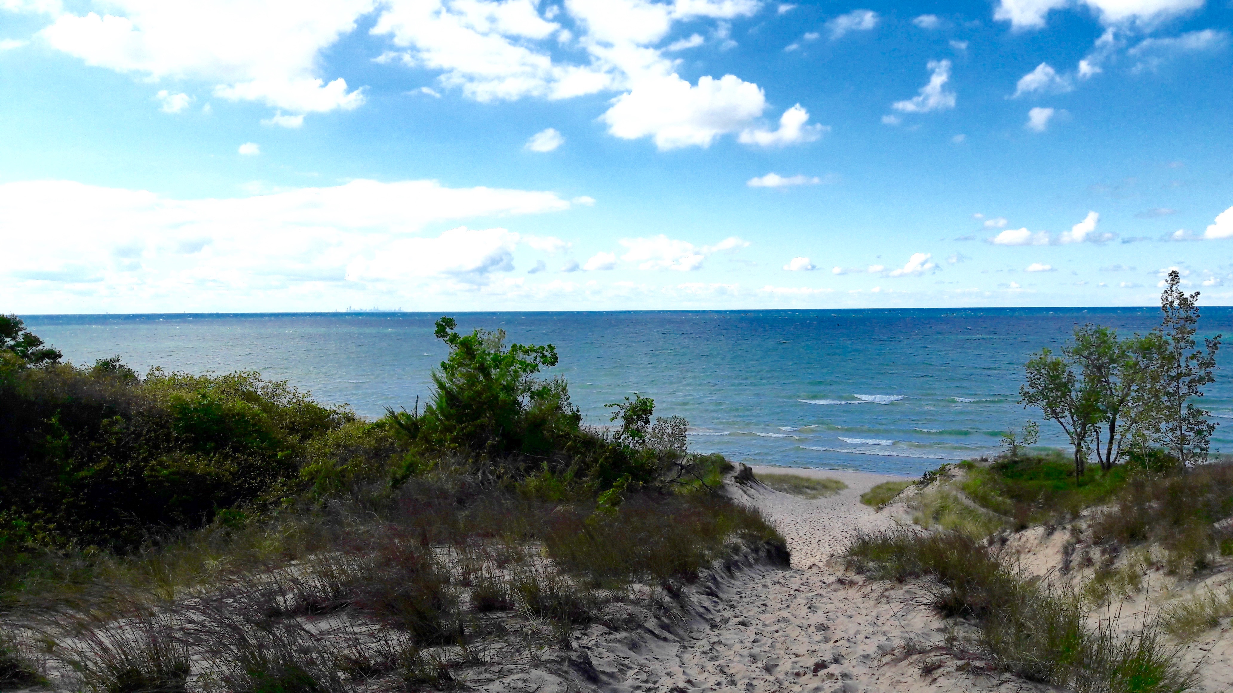 Photo number 3
 Photo number 4
 Photo number 5
 Photo number 6
 Photo number 7
 Photo number 8
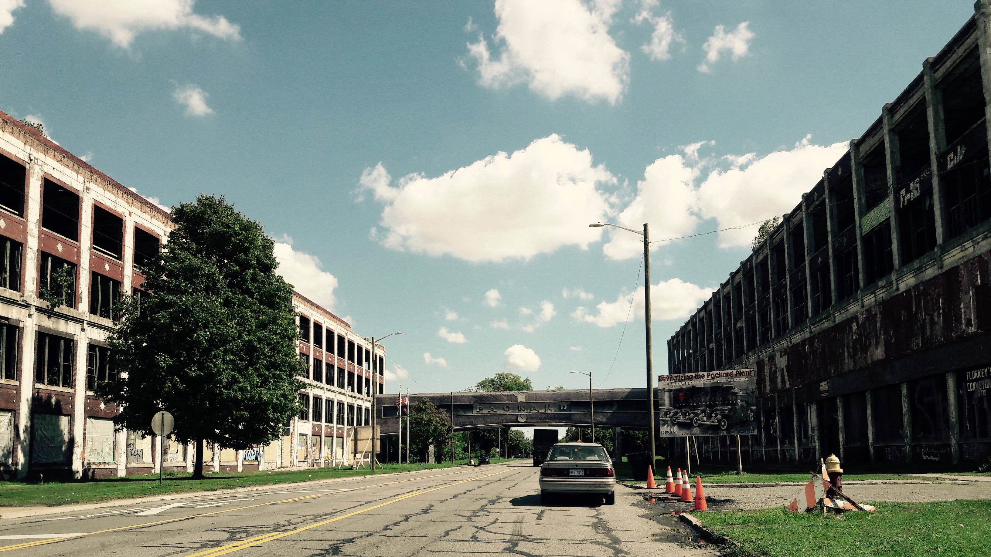 Photo number 9
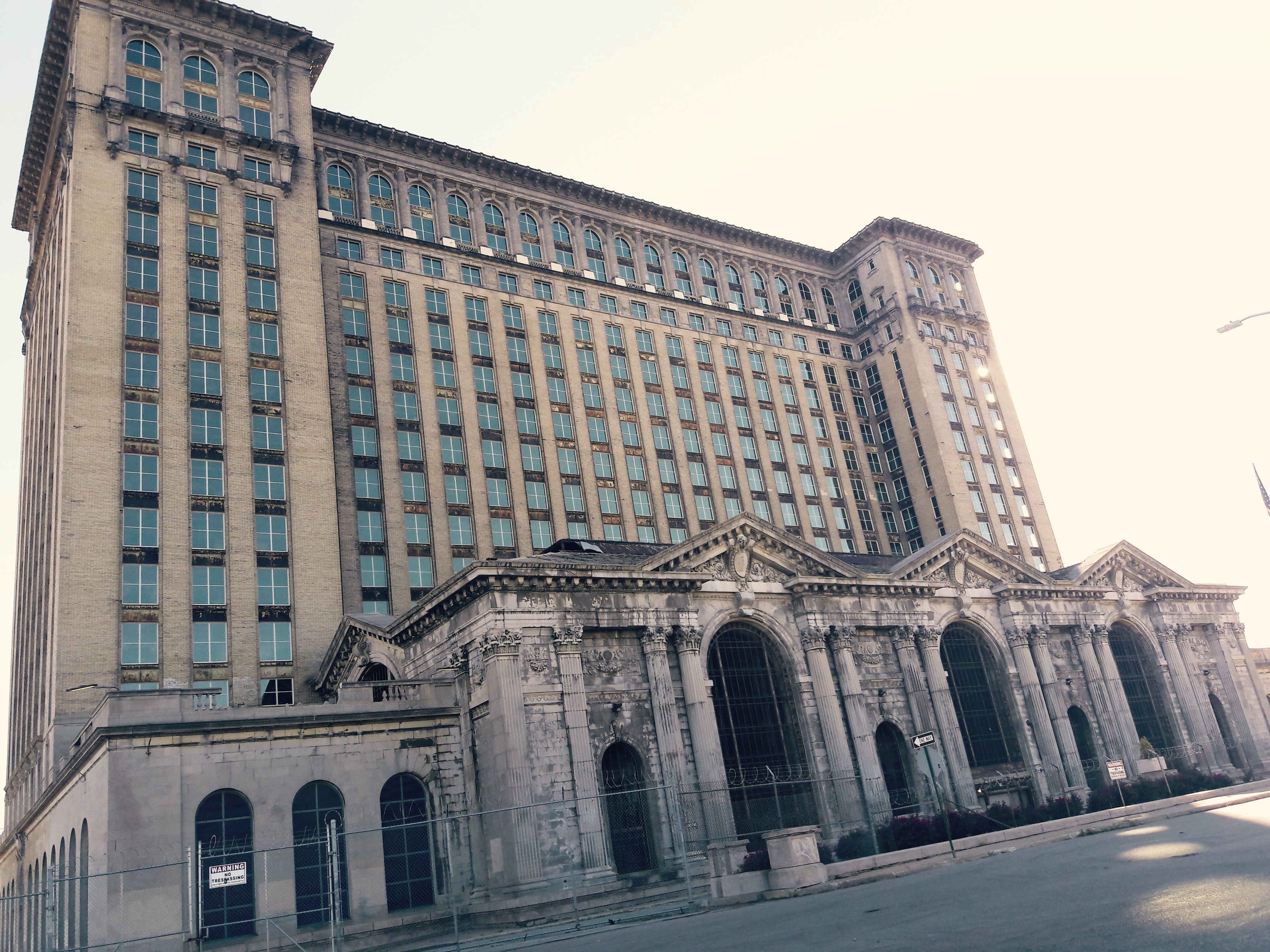 Photo number 10
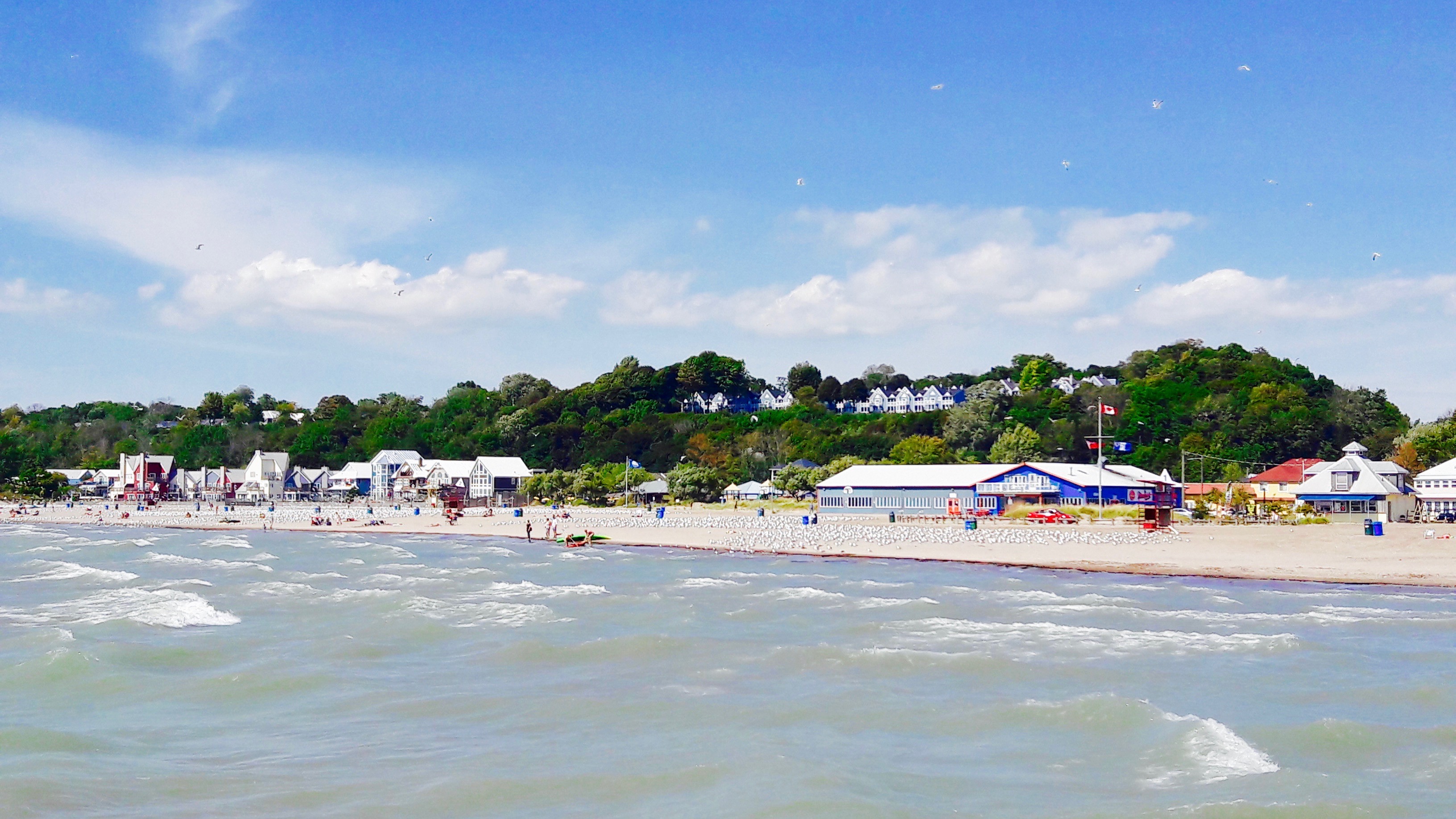 Photo number 11
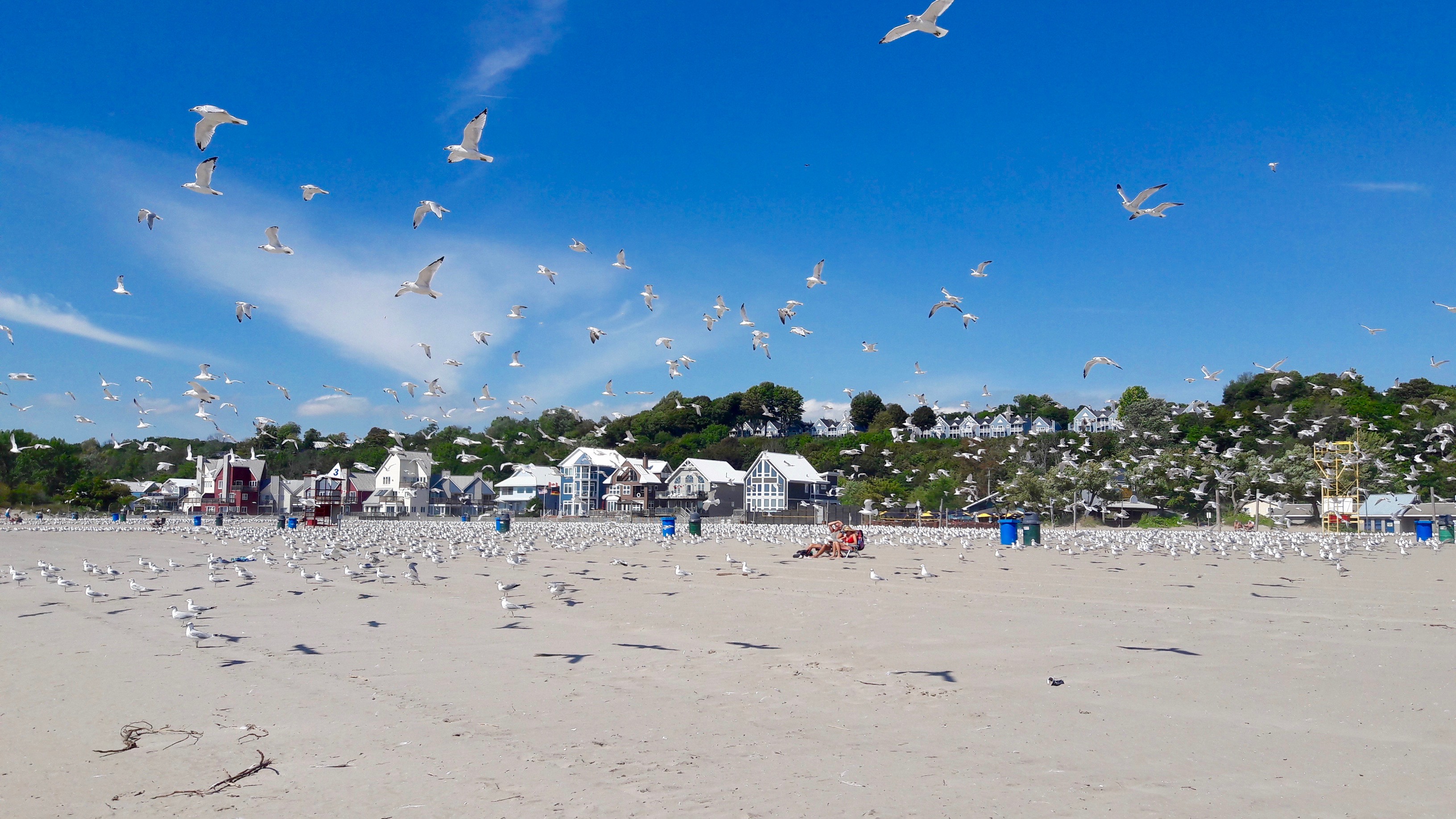 Photo number 12
 Photo number 13
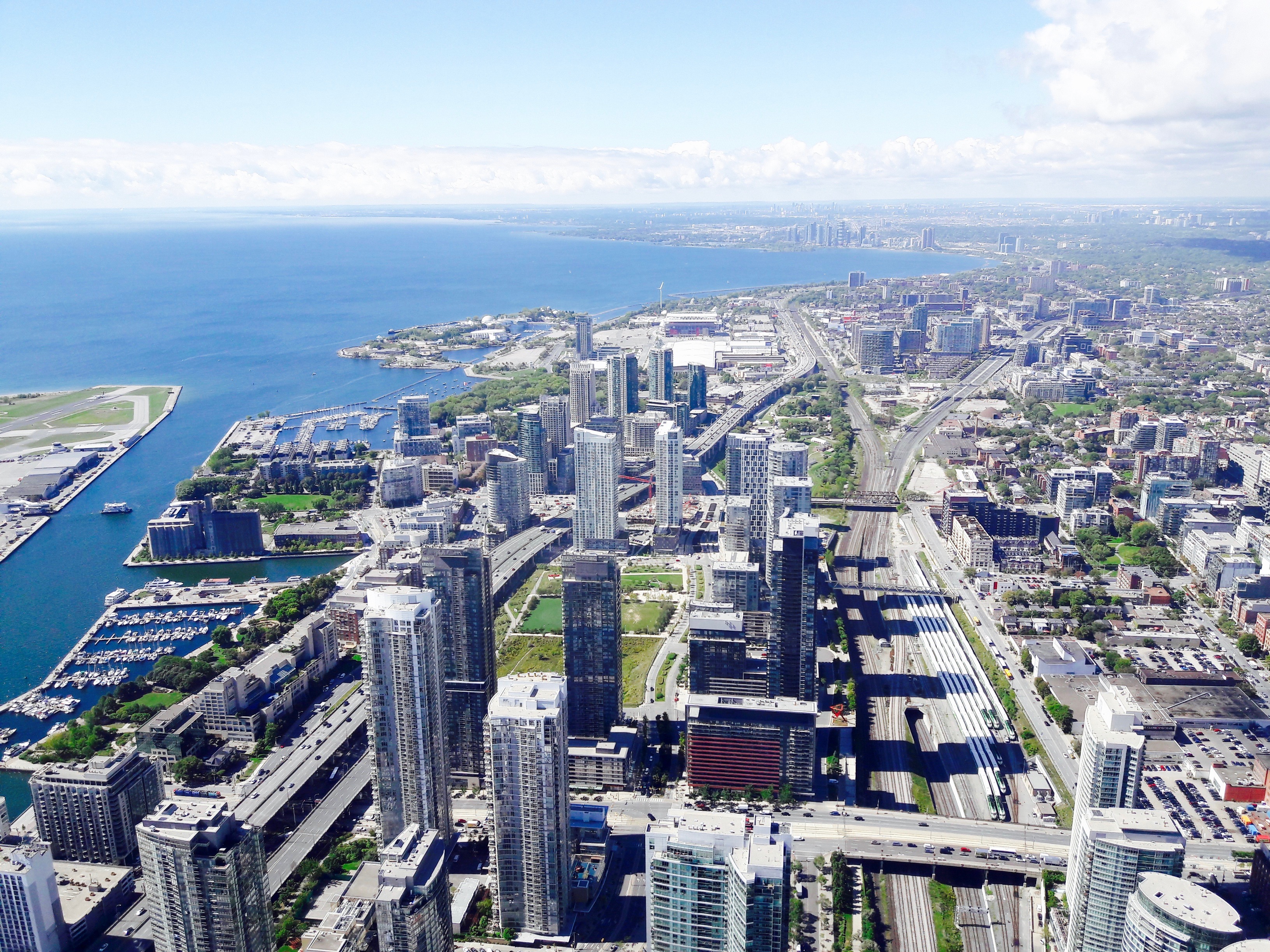 Photo number 14
 Photo number 15
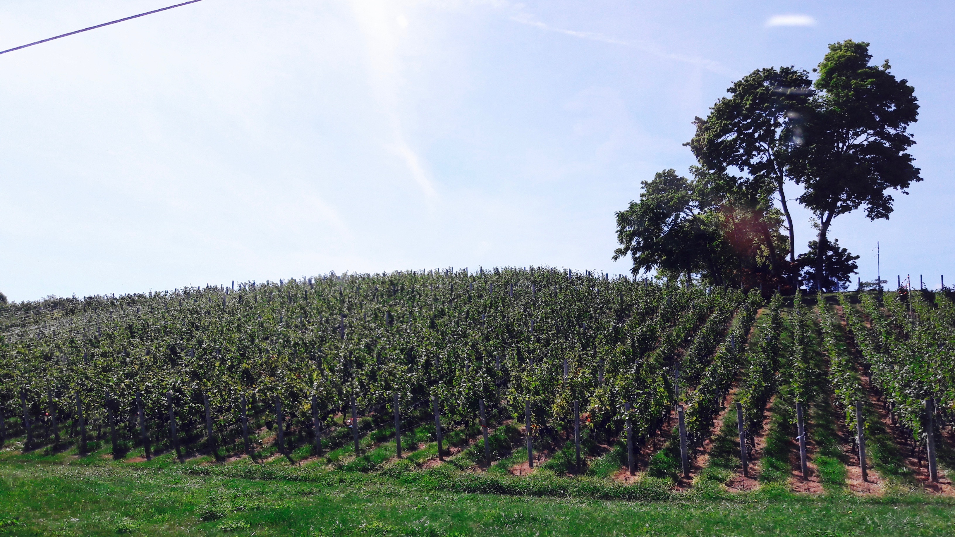 Photo number 16
 Photo number 17
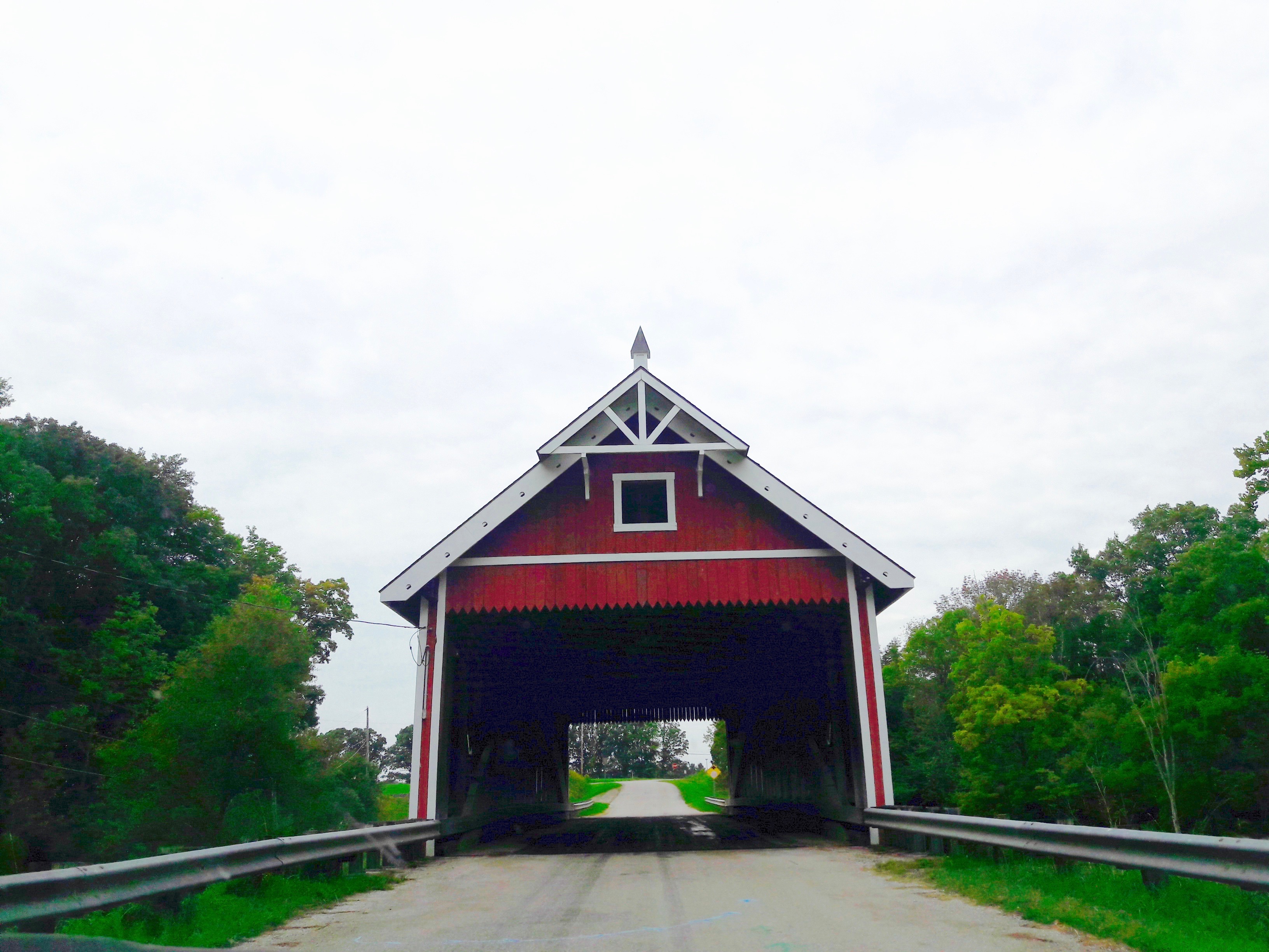 Photo number 18
 Photo number 19
 Photo number 20
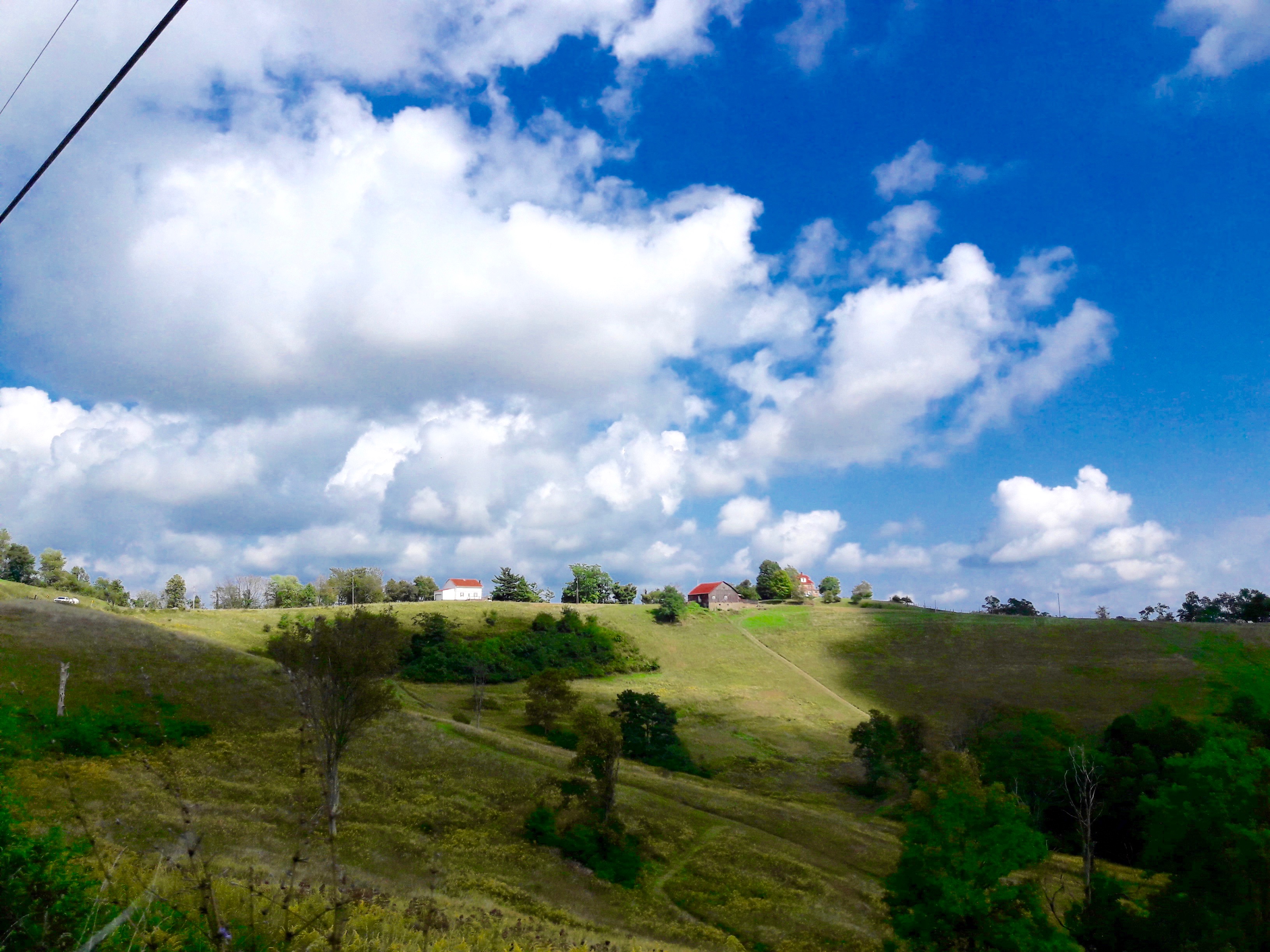 Photo number 21
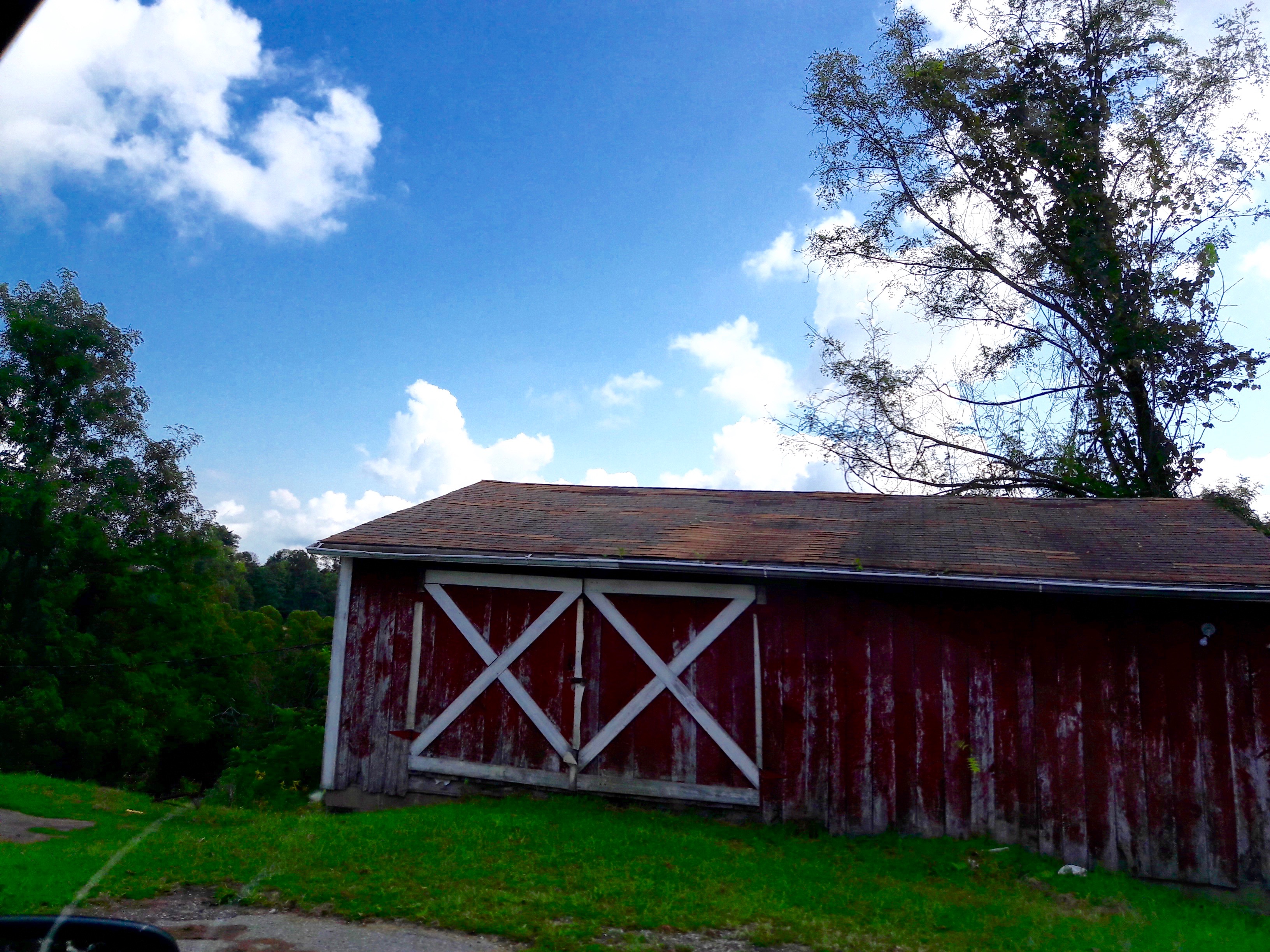 Photo number 22
 Photo number 23
 Photo number 24
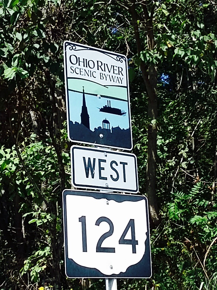 Photo number 25
 Photo number 26
 Photo number 27
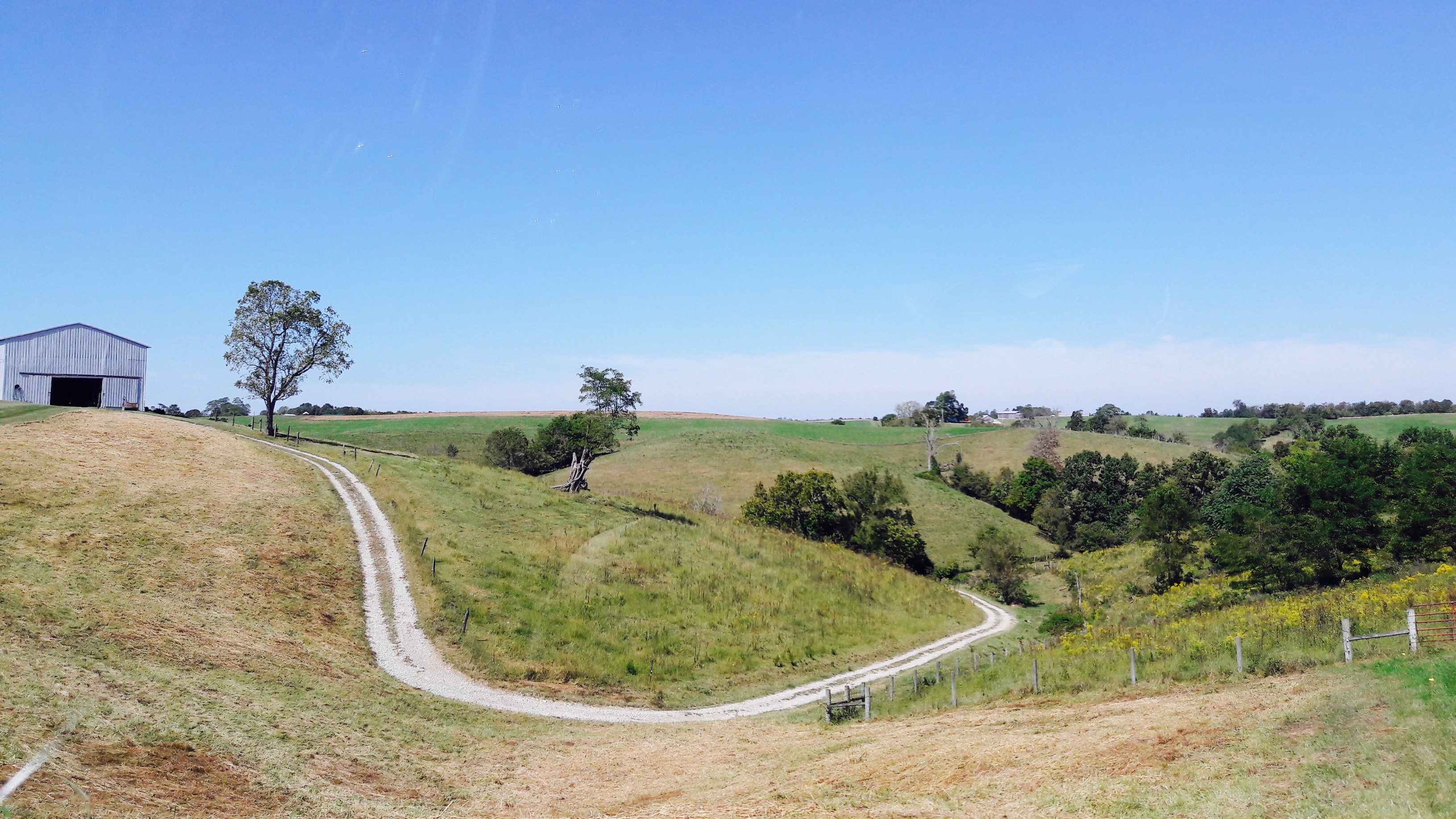 Photo number 28
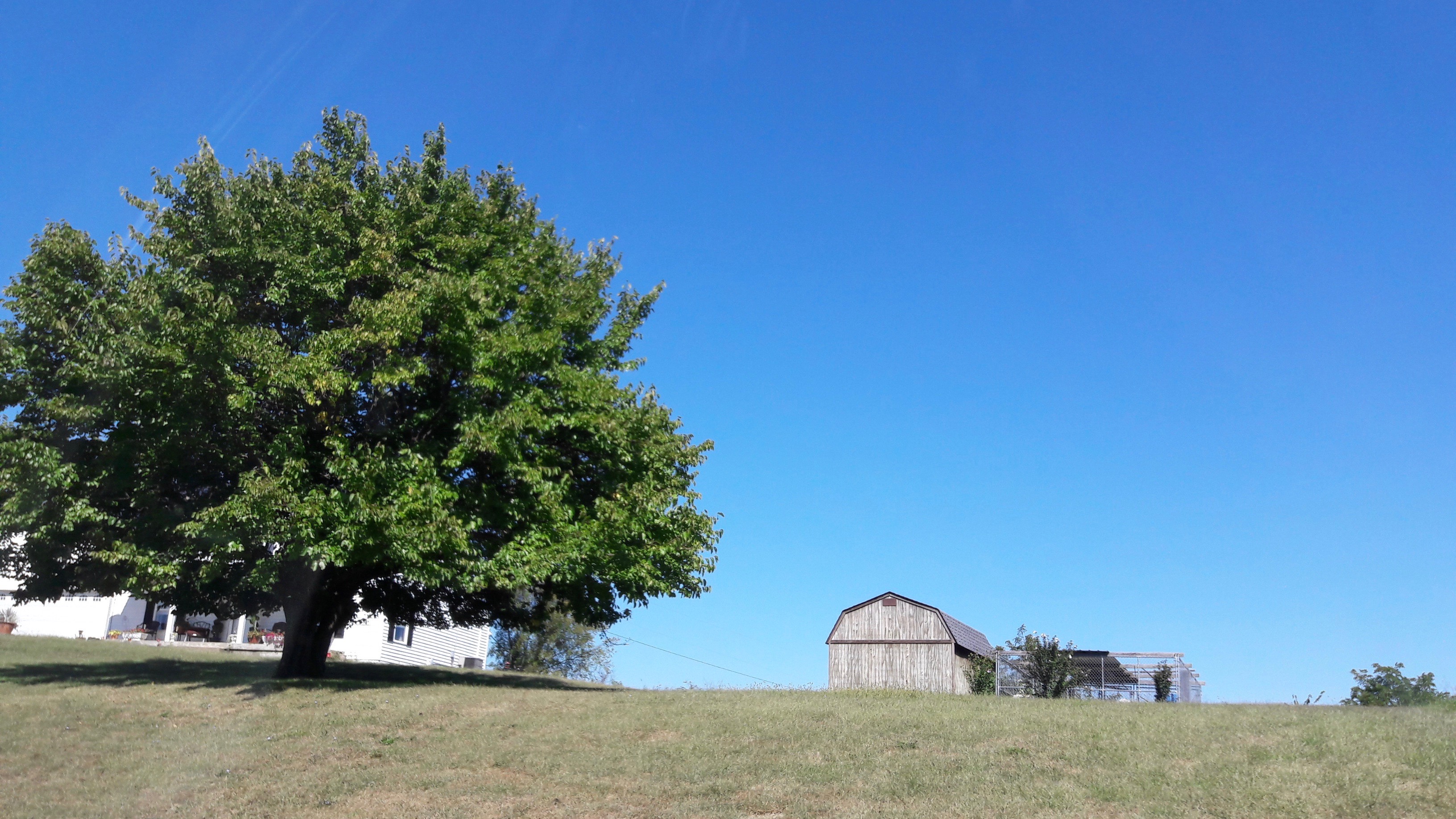 Photo number 29
 Photo number 30
 Photo number 31
 Photo number 32
 Photo number 33
 Photo number 34
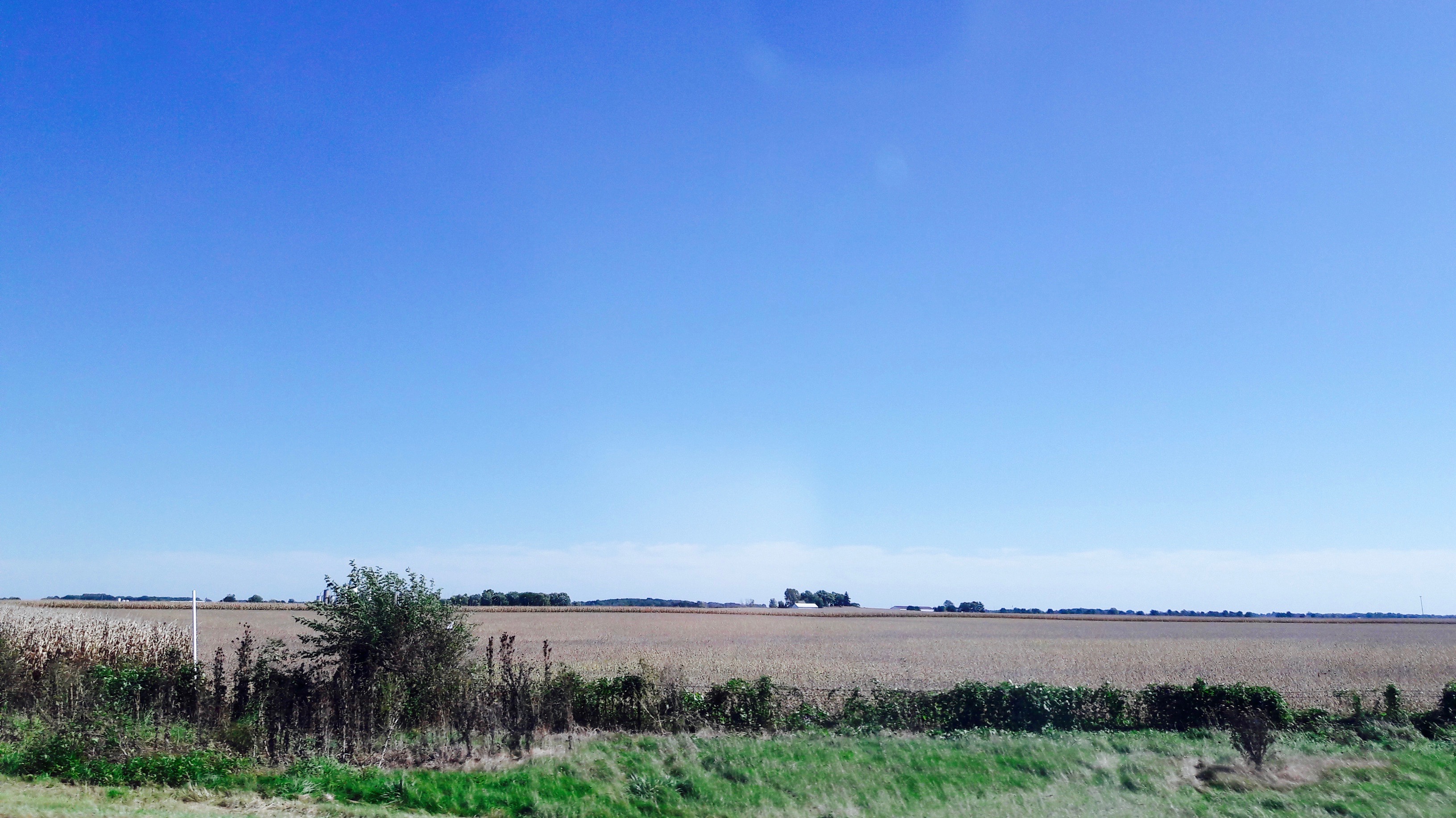 Photo number 35
